One of the primary concerns that roboticists have when considering technologies for real-time control is the predictability of latency. The worst case latency tends to be more important than the overall throughput, so the possibility of latency spikes and packet loss in a communication standard represent significant red flags.

Much of the prevalent hesitance towards using Ethernet for real-time control originated in the early days of networking. Nodes used to communicate over a single shared media that employed a control method with random elements for arbitrating access (CSMA/CD). When two Frames collided during a transmission, the senders backed off for random timeouts and attempted to retransmit. After a number of failed attempts, frames could be dropped entirely. By connecting more nodes through Hubs the Collision Domain was extended further, resulting in more collisions and less predictable behavior.

In a process that started in 1990, Hubs have been fully replaced with Switches that have dedicated full-duplex (separate lines for transmitting and receiving) connections for each port. This separates segments and isolates collision domains, which eliminates any collisions that were happening on the physical (wire) level. CSMA/CD is still supported for backwards compatibility and half-duplex connections, but it is largely obsolete.

Using dedicated lines introduces additional buffering and overhead for forwarding Frames to intended receivers. As of 2016, virtually all Switches implement the Store-and-Forward switching architecture in which Switches fully receive packets, store them in an internal buffer, and then forward them to the appropriate receiver port. This adds a latency cost that scales linearly with the number of Switches that a packet has to go through. In the alternative Cut-through approach Switches can forward packets immediately after receiving the target address, potentially resulting in lower latency. While this is sometimes used in latency sensitive applications, such as financial trading applications, it generally can’t be found in consumer grade hardware. It is more difficult to implement, only works well if both ports negotiate the same speed, and requires the receiving port to be idle. The benefits are also less significant on smaller packets due to the requirement to buffer enough data to evaluate the target address.

Another problem that many roboticists are often concerned about is Out-of-Order Delivery, which means that a sequence of packets coming from a single source may be received in a different order. This is relevant for communicating over the Internet, but generally does not apply to local networks without redundant routes and load balancing. Depending on the driver implementation it can theoretically happen on a local network, but we have yet to observe such a case.

There are several competing networking standards that are built on Ethernet and can guarantee enough determinism to be used in industrial automation (Industrial Ethernet). They achieve this by enforcing tight control over the network layout and by limiting the components that can be connected. However, even cheap consumer grade network equipment can produce very good results if the network is controlled in a similar manner.

Note that this is not a new concept. We found several resources that discussed similar findings more than a decade ago, e.g., Real-Time-Ethernet (2001), Real-time performance measurements using UDP on Windows and Linux (2005), Evaluating Industrial Ethernet (2007), and Deterministic Networking: from niches to the mainstream (2013).

A common way to benchmark networks is to setup two computers and have a sender transmit a message to a receiver that echoes it back. That way the sender can measure the round-trip time (RTT) and gather statistics of the network. This generally works well, but large operating system stacks and device drivers can potentially add a lot of variation. In an attempt to reduce unwanted jitter, we decided to setup a benchmark using two embedded devices instead.

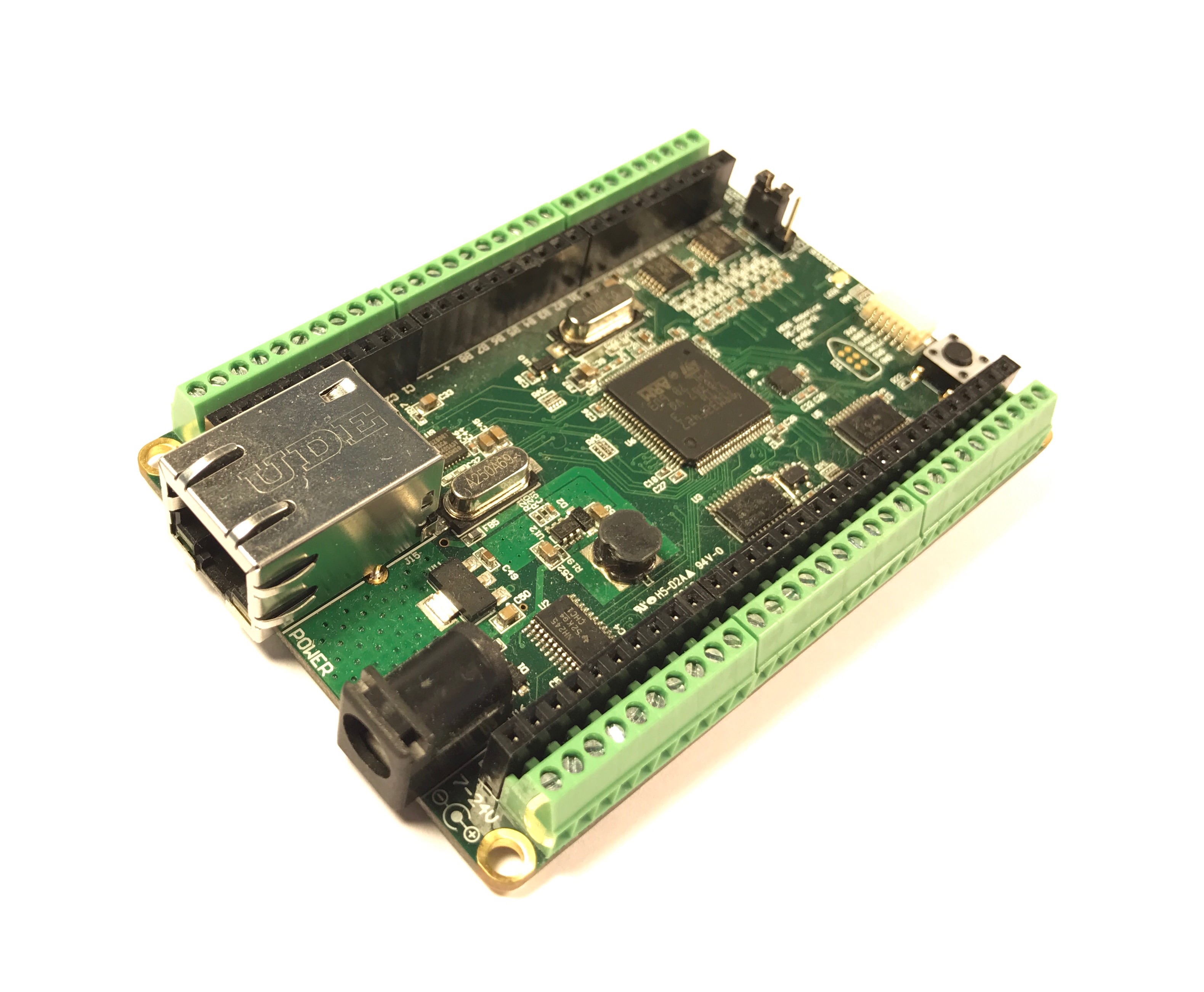
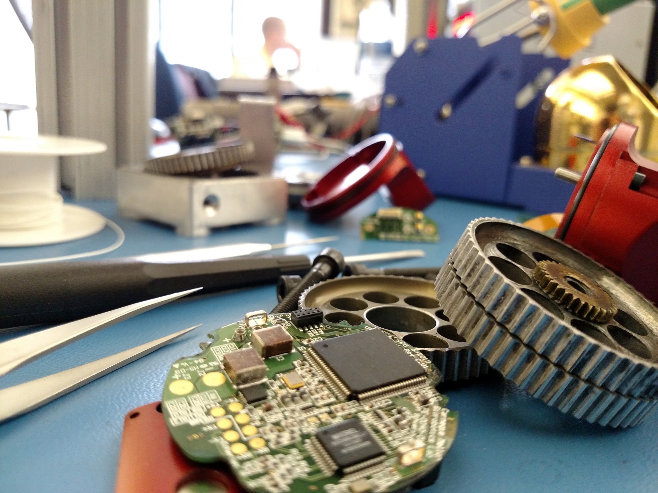
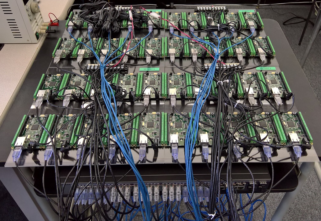
Our startup HEBI Robotics builds a variety of building blocks that enable quick development of custom robotic systems. We mainly focus on actuators, but we’ve also developed other devices such as the I/O Board shown in the picture above. Each board has 48 pins that serve a variety of functions (analog and digitial I/O, PWM, Encoder input, etc.) that can be accessed remotely via network. We normally use them in conjunction with our actuators to interface with external devices, such as a gripper or pneumatic valve, or to get various sensor input into MATLAB.

Each device contains a 168MHz ARM microcontroller (STM32f407) and a 100 Mbit/s network port, so we found them to be very convenient for doing network tests. We selected two I/O Boards to act as the sender and receiver nodes and developed custom firmware in order to isolate the network stack. The resulting firmware was based on ChibiOS 2.6.8 and lwIP 1.4.1. The relevant code pieces can be found here. The elapsed time was measured using a hardware counter with a resolution of 250ns.

Since there was no way to store multiple Gigabytes on these devices, we decided to log data remotely using a UDP service that can receive measurement data and persist to disk (see code). In order to avoid stalls caused by disk I/O, the main socket handler wrote into a double buffered structure that got persisted by a background thread. The synchronization between the threads was done using a WriterReaderPhaser, which is a synchronization primitive that allows readers to flip buffers while keeping writers wait-free. We found this primitive to be very useful for persisting events that are represented by small amounts of data.

The step by step flow was as follows:

The resulting binary data was loaded into MATLAB© for analysis and visualization. The code for reading the binary file can be found here.

The round-trip time is the difference between the receive and transmit timestamps. We also recorded the sequence number of each packet and the ip address of the receiver node in order to detect packet loss and track ordering.

UDP datagrams include a variety of headers that result in a minimum of 66 bytes of overhead. Additionally, Ethernet Frames have a minimum size of 84 bytes, which makes the minimum payload for a UDP Datagram 18 bytes. The rough structure is shown below. More detailed information can be found at Ethernet II, Internet Protocol (IPv4), and User Datagram Protocol (UDP).

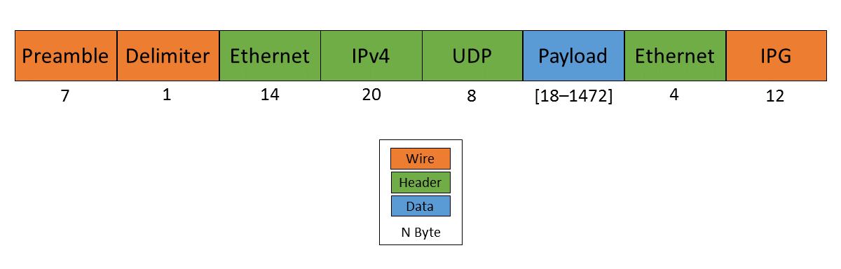
Although this overhead may seem high for traditional automation applications with small payloads (<10 bytes), it quickly amortizes when communicating with smarter devices. For example, each one of our X-Series actuators contains more than 40 sensors (position, velocity, torque, 3-axis gyroscope, 3-axis accelerometer, several temperature sensors, etc.) that get combined into a single packet that uses between 185 and 215 bytes payload. Typical feedback packets from an I/O Board are even larger and require about 300 bytes. When comparing overhead it is also important to consider the available bandwidth, i.e., as sending 100 bytes over Gigabit Ethernet (even over 100 Mbit/s) tends to be faster than sending a single byte using traditional non-Ethernet based alternatives such as RS485 or CAN Bus.

For these benchmarks we chose to measure the round-trip time for a payload of 200 bytes. After including all overhead, the actual size on the wire is 266 bytes. The theoretical time it takes to transfer 266 bytes over 100 Mbit/s and 1Gbit/s Ethernet is 20.3us and 2.03us respectively.

Note that while the size is representative of a typical actuator feedback packet, the round-trip times in production may be faster because outgoing packets (commands) tend to be significantly smaller than response packets (feedback).

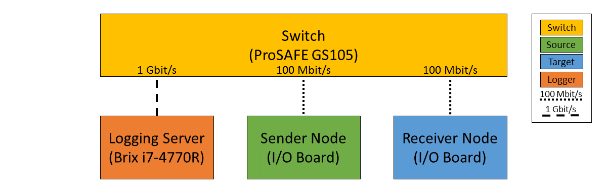
We can establish a baseline of the best-case round-trip time by having the sender and receiver nodes communicate with each other through a single Switch that does not see any external traffic. We did not setup a point-to-point connection without any Switches because the logging server needed to be on the same network and because we rarely see this case in practice.

We set the frequency to 100Hz and logged data for ~24 hours. We chose this frequency because it is a common control rate for sending high-level trajectories, and because 10ms is a safe deadline in case there are large outliers. During normal operations we typically used rates between 100-200Hz for updating set targets of controllers that get executed on-board each device (e.g. position/velocity/torque), and rates of up to 1KHz when bypassing local controllers and remotely controlling the output (e.g. PWM). The network would technically support even higher rates, but there are usually other limitations that come into play at around 1KHz (e.g. OS scheduler and limited sensor polling rates).

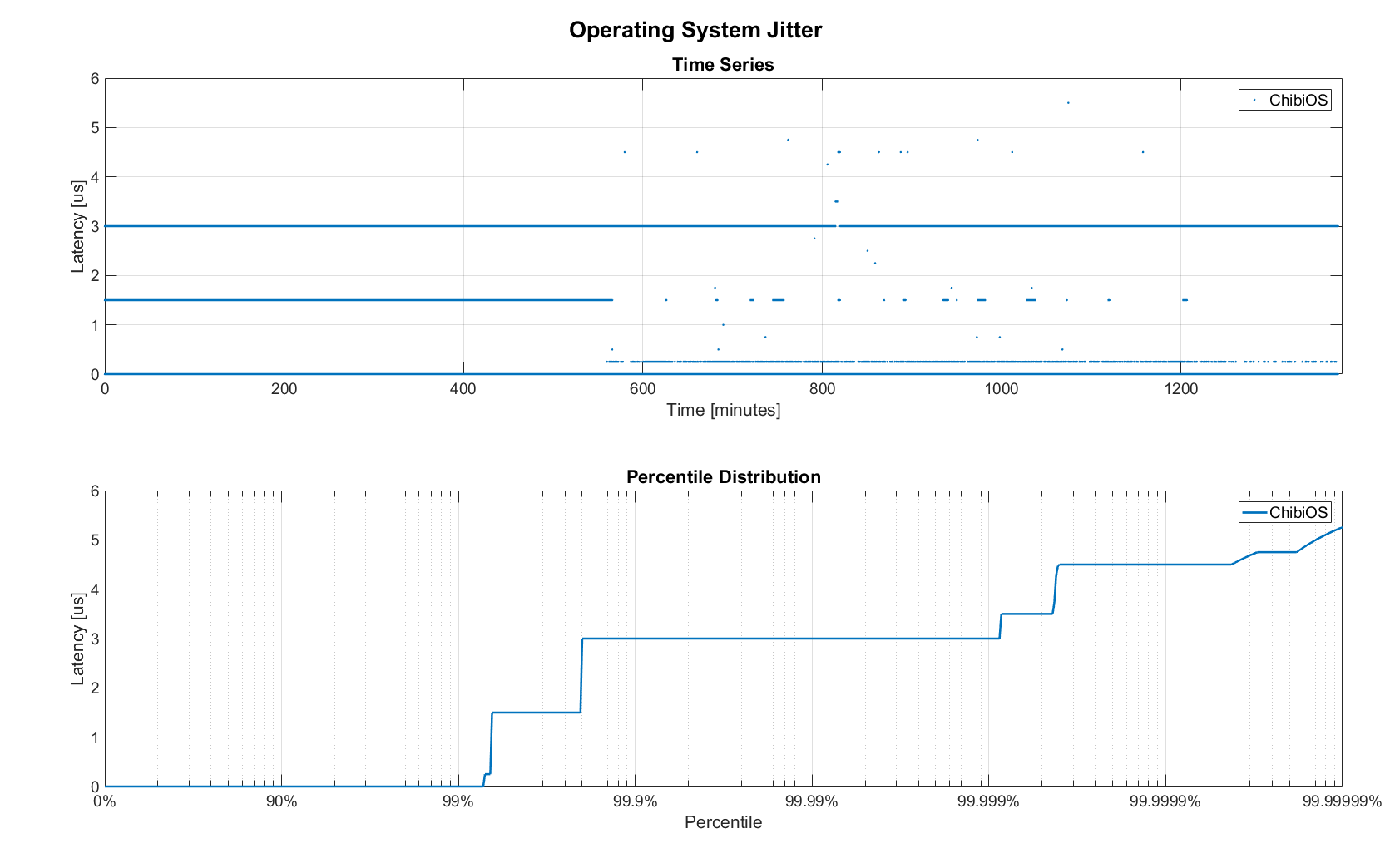
First, we looked at the jitter of the underlying embedded real-time operating system (RTOS). The figure below shows the difference between an idealized signal that ticks every 10ms and the measured transmit timestamps. 99% are within the lowest measurement resolution (250ns), and the total observed range is slightly below 6us. Note that this is significantly better than the 150us base jitter range we observed on real-time Linux (see The Importance of Metrics and Operating Systems).

The two figures below show the round-trip time for all packets and the corresponding percentile distribution. There were a total of 8.5 million messages. None of them were lost and none of them arrived out of order.

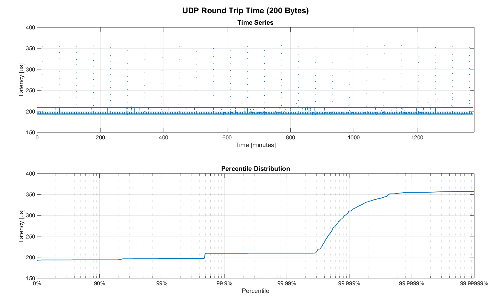
90% of all packets arrived within 194us and a jitter of less than 1 microsecond. Roughly 80us of this time was spent on the wire, so using chips that support Gigabit (rather than 100Mbit) could lower the round-trip time to ~120us. Above the common case, there were three different periodically reoccuring modes that resulted in additional latency.

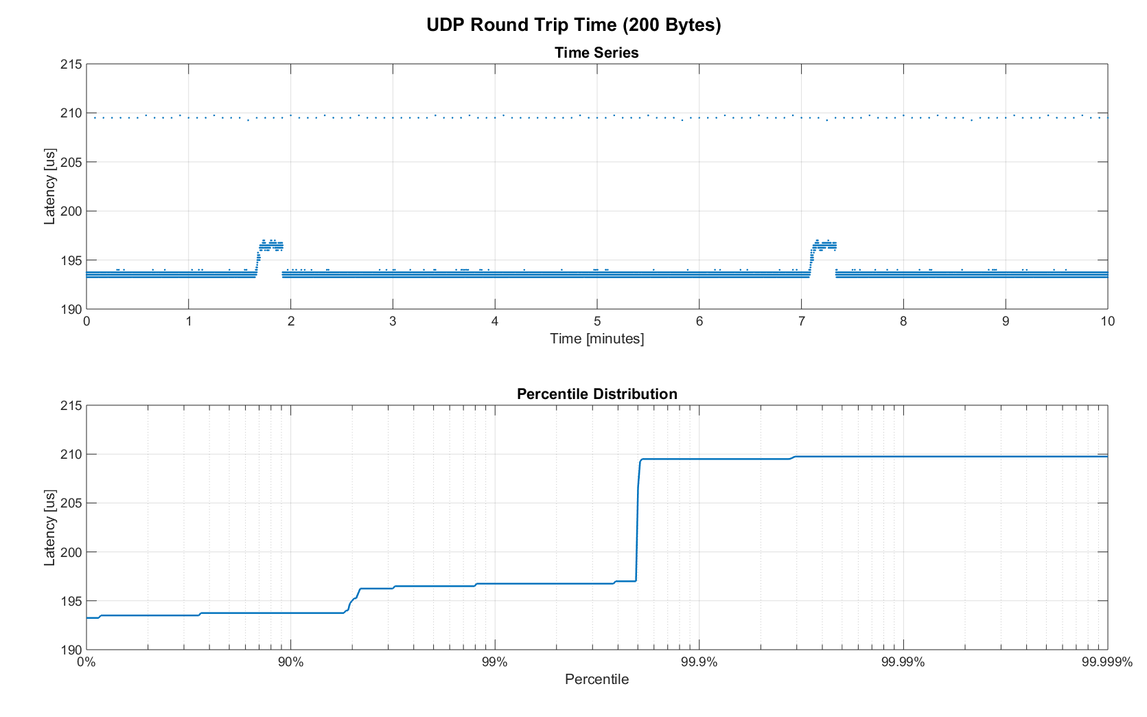
The zoomed in view of a 10 minute time span highlights Modes 1 and 2. All three modes seemed to be related to actual time and independent of rate and packet count. We were unable to find the root cause of these modes, but after several tests we strongly suspected that all of them were caused by the programmed firmware rather than being tied to the Switch or the actual protocol.

Overall this initial data looked very promising for being able to use UDP for many real-time control tasks. With more tuning and a better implementation (e.g. lwip with zero copy and tuned options) it seems likely that the maximum jitter could be reduced to below 6us and maybe even below 1us.

As mentioned in the background section, most modern Switches use the 'store-and-forward' approach that requires the Switch to fully receive a packet before forwarding it appropriately. Therefore, the latency cost per Switch is the time a packet spends on the wire plus any switching overhead. The wire time is constant (2.03us or 20.3us for 266 bytes), but the overhead depends on the Switch implementation. It can be difficult to find good performance data for specific devices, so depending on your requirements you may need to conduct your own benchmarks if you need to evaluate hardware.

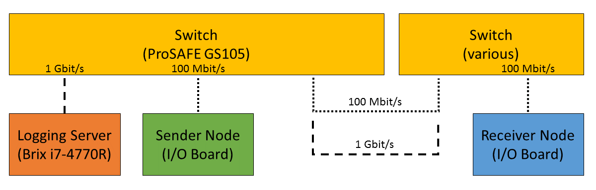
For this benchmark we tested the three following Switches and added them individually to the baseline setup as shown above,

In total there were about 1 million packets. Again, we did not observe any packet loss or out-of-order delivery.

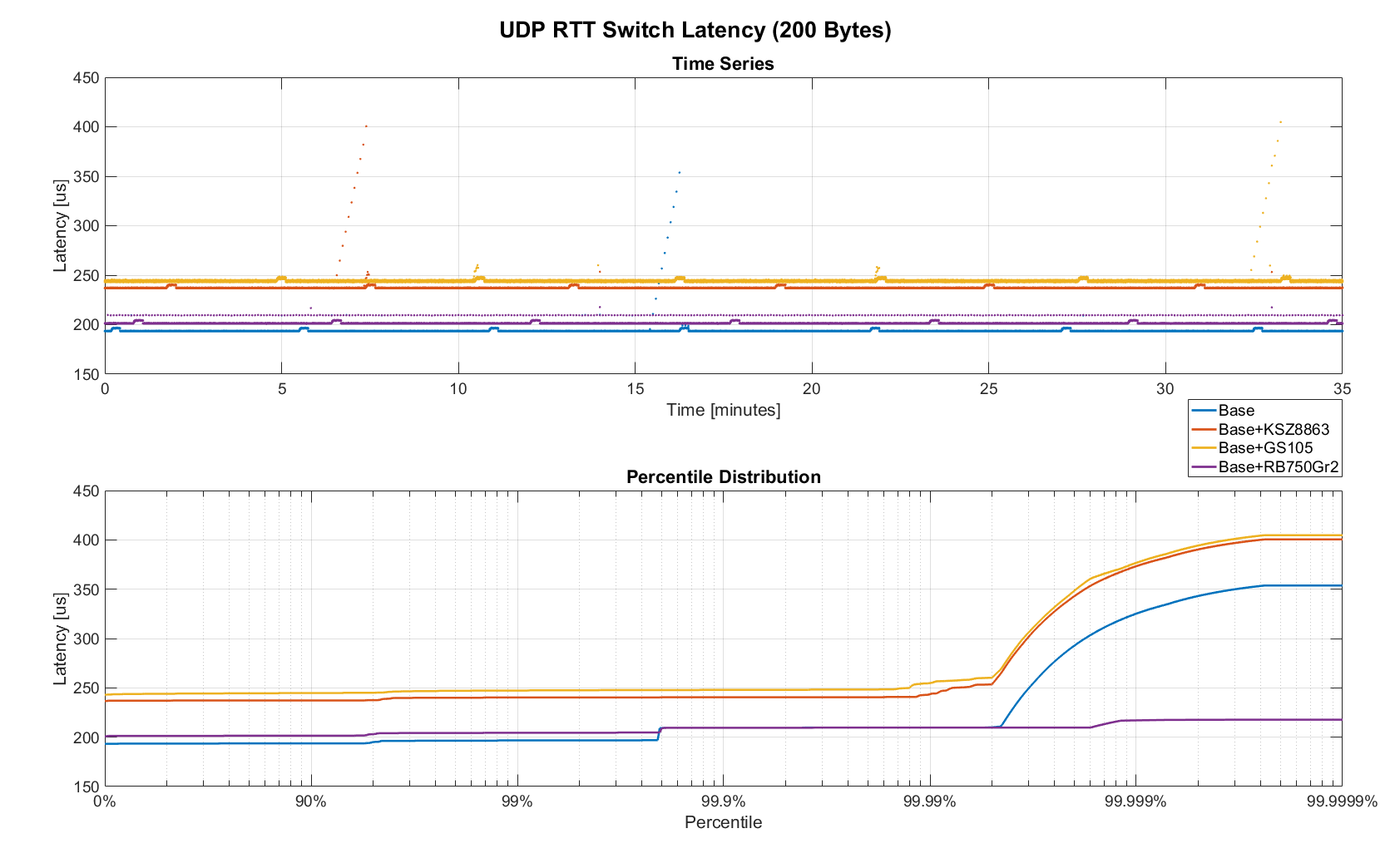
The figure below shows a zoomed view of the time series highlighting the added jitter characteristics. Modes 1 and 3 do not seem to be affected by additional switches. Mode 2 remains constant at 210 us and disappears for higher round-trip times, indicating an issue at the receiving step of the sender.

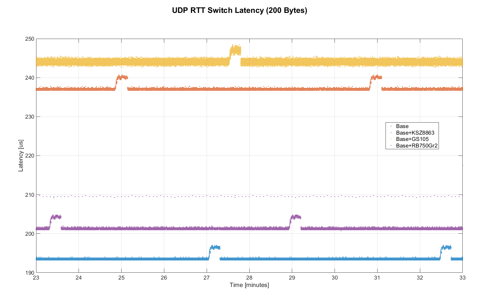
Both KSZ8863 and the RB750Gr2 add a constant switching latency of 2.9 us and 3.6 us in addition to the wire time of 40.6 us and 4.06 us respectively to the RTT. The added jitter seems to be negligible at well below 1us. Surprisingly, the GS105 seems to have problems with this use case, resulting in higher latency and more jitter than the KSZ8863 even though it was connected using Gigabit. More details are in the table below.

According to the GS105 spec sheet, the added network latency should be below 10us for 1 Gbit/s and 20us for 100 Mbit/s connections. We did additional tests and the GS105 did seem to perform according to spec when using exclusively 100 Mbit/s or 1 Gbit/s on all ports.

We also conducted another baseline test that replaced the GS105 with a RB750Gr2. While we found a consistent improvement of 0.5us, we did not consider this significant enough to rerun all tests.

So far all tests were measuring the round-trip time between a sender node and a single target node. Since real robotic systems can contain many devices, e.g., one per axis or degree of freedom, we also looked at how UDP performs with multiple devices on the same network. In conversations with other roboticists we often found an expectation that there would be significant packet loss if multiple packets were to arrive at a Switch at the same time. The worst case would occur if all devices were connected to a single Switch as shown below.

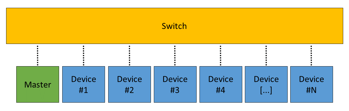
In order to test the actual behavior we setup a test consisting of 40 HEBI Robotics I/O boards that were connected to a single 48-port Ethernet Switch (GS748T). All devices were running the same (receiver) firmware as before, so sending a single broadcast message triggered 40 response packets that caused more than 10 KB of total traffic to arrive at the Switch within occasionally less than 250 nanoseconds. These Microbursts were well beyond the sustainable bandwidth of Gigabit Ethernet. The setup shown below was representative of a high degree of freedom system such as a full body humanoid robot without daisy-chaining.

We would also like to mention that this setup heavily benefited from two side effects of using a standard Ethernet stack. First, there was no need for any manual addressing because of DHCP and device specific globally unique mac addresses. Second, we were able to re-program the firmware on all 40 devices simultaneously within 3-6 seconds due to the fact that we had a bootloader with TCP/IP support. It would have been very tedious to setup such a system if any step had required manual intervention.

Since the combined responses resulted in more load than the sender device was able to easily handle, we exchanged the sender I/O Board with a Gigabyte Brix i7-4770R desktop computer running Scientific Linux 6.6 with a real-time kernel. We setup the system as described in The Importance of Metrics and Operating Systems and disabled the firewall.

Running the benchmark at 100Hz for ~90 minutes resulted in more than 20 million measurements.

Again, we first looked at the jitter of the underlying operating system. The figure below shows the difference between an idealized signal that ticks every 10ms and the measured transmit timestamps. It shows that this setup suffers from more than an order of magnitude more jitter than the embedded RTOS. Note that the corresponding jHiccup control chart looks identical as in the OS blog post.

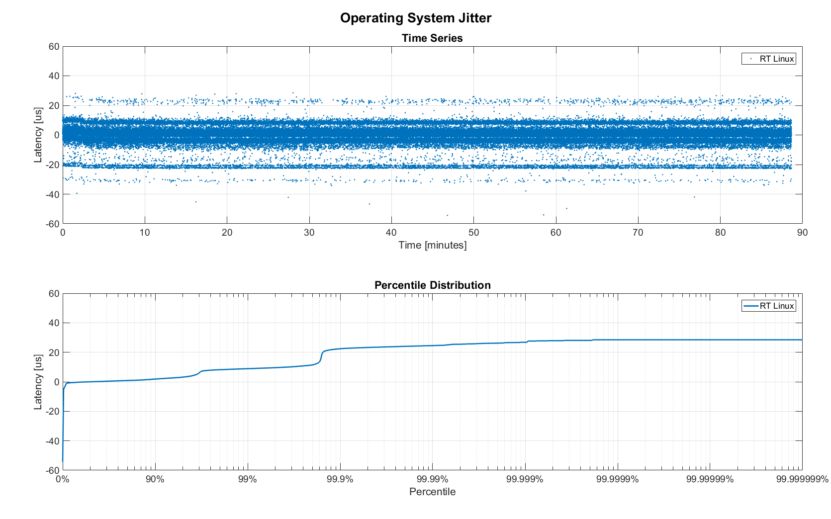
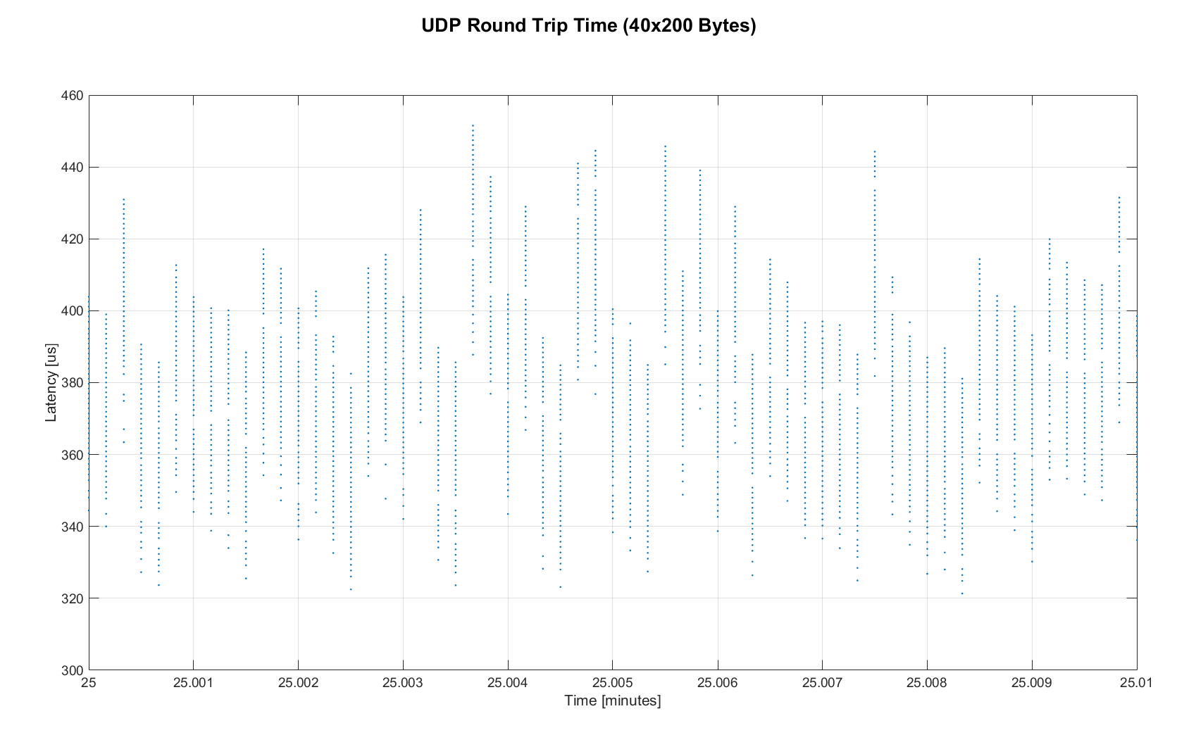
The two figures below show the round-trip time for each measurement. It may be surprising, but there was again no packet loss or re-ordering of packets from any single source.

Rather than packets being dropped, what actually happened was that all packets were stored in the internal 1.6 MB buffer of the switch, queued, and forwarded to the target port as fast as possible. Since the sender was connected via Gigabit, the packets arrived roughly every ~2us. The time axis in the chart is based on the transmit timestamp, so each cycle shows up as vertical column in the graphs. We also conducted the same test at 1KHz and found identical results.

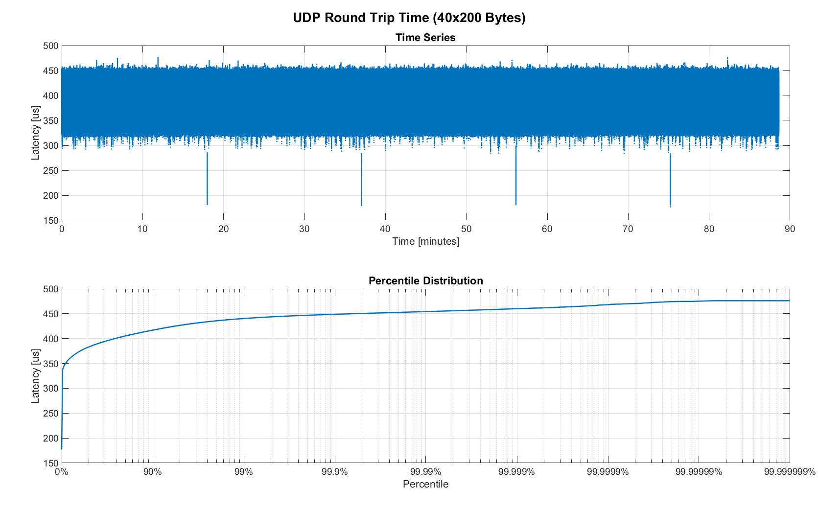
However, the amount of latency and jitter turned out to be worse than we anticipated. We expected most columns to start at around ~180us and end at ~280us. While this was sometimes the case, the majority of columns started above 300 us. After some initial research we suspected that this delay was mostly caused by the Linux NAPI using polling mode rather than interrupts, and by using a low-cost network interface paired with suboptimal device drivers. While we expected the OS and driver stack to introduce additional latency and jitter, we were surprised by the order of magnitude.

The installed network interface and driver are below.

03:00.0 Ethernet controller: Realtek Semiconductor Co., Ltd. RTL8111/8168/8411 PCI Express Gigabit Ethernet Controller (rev 0c)

r8169 Gigabit Ethernet driver 2.3LK-NAPI loaded

Even consumer-grade Ethernet networks can exhibit very deterministic performance with regards to latency. In the more than 100 million packets that were sent for this blog post, we did not observe any packet loss or out-of order delivery. Even when communicating with 40 smart devices that represent a total of 1.600 sensors at a rate of 1KHz we found the network to be very reliable. While we still believe that large and dangerous industrial robots should be controlled using specialized industrial networking equipment, we feel that standard UDP is more than sufficient for most robotic applications.

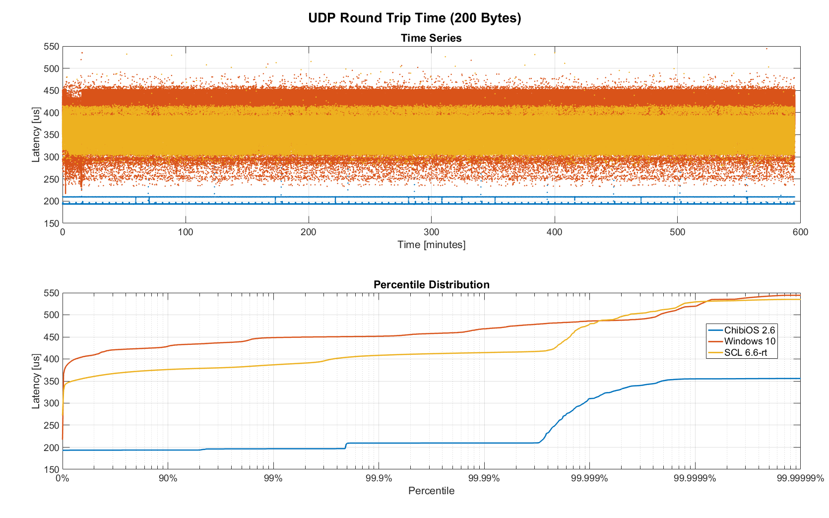
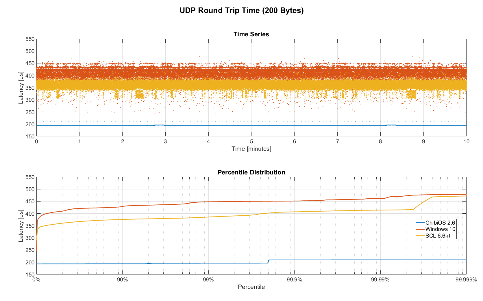
We also found that most of the observed latency and jitter were caused by the underlying operating systems and their device drivers. To further illustrate this point we did additional comparisons of the baseline setup with the sender node running on different operating systems. The configurations were as follows:

The two charts below show the round trip time for each system communicating with a single I/O Board over a single Switch. Note that Linux and Windows were connected to the Switch via Gigabit and should have received datagrams ~40us before the embedded device.

We realize that there are many more interesting questions that were beyond the scope of this work. We are currently considering the following networking-related topics for future blog posts:

If there are other topics that you think would be worth covering, please leave a note in the comment section. If you are working for a hardware vendor that specializes in low-latency networking equipment and would be willing to provide samples for evaluation, please contact us through our website.